Money Talks:Understanding Mean, Mode, Median, Standard Deviation, and Variance and their relationship to your finances.

Introduction

You have probably heard of these terms; Mean, Mode, and Median, and perhaps even used them in school. But you may never have stopped to think about what they truly mean for your everyday life. You may have also tried generating a report at mpesa-summary section, or summarise-statements section, or transactions section after uploading your M-Pesa statement and seen a summary full of these numbers, only to wonder: why does any of this matter to me? This is a sample image obtained from the statistics section of the MPecunia report;

The truth is, these are not just classroom concepts. They are powerful measures used by some of the world's most successful companies to drive real decisions. Take Coca-Cola, for example, the company spent approximately $5 billion on advertising in 2023 alone. But that spend is not distributed evenly across all markets. The budget allocated to, say, the Middle East versus North America is informed by layers of statistical analysis. This is one of the key areas where many Western companies hold an advantage over their counterparts in Africa: they make decisions grounded in data, not just intuition or the presence of revenue.

And with MPecunia, we believe that kind of thinking should be accessible to everyone, including you. So let us start with the basics, and build up to why these statistical measures matter deeply when it comes to your personal and business finances.

Two Types of Statistics

Before we dive in, it helps to understand that statistics can be divided into two broad categories:

1. DESCRIPTIVE STATISTICS

This involves summarizing and organizing data you already have; turning it into charts, tables, and summaries that are easy to understand and communicate. Think of it as telling the story of your data. The statistical measures we cover in this article, Mean, Mode, and Median, fall under what is called Measures of Central Tendency. They are tools for describing what is 'typical' in a dataset.

Example: Imagine you open a shoe business and record every sale in a book/ledger. When you eventually sit down to analyze that ledger, you are doing descriptive statistics. You get to ask: How much money do I make on average each month? Which shoe sells the most? What does a typical day's profit look like? The data answers all of these questions.

2. INFERENTIAL STATISTICS

From the word 'infer,' you can already guess what this involves; using a sample of your data to draw conclusions and make predictions about a larger picture. It is, in a way, playing the role of a well-informed prophet.

Example: Going back to the shoe business; if you find that Crocs are your best seller in shops A, D, and G out of shops A through J, you might decide to restock Crocs across all your branches. That decision is inferential statistics in action. There are formal mathematical tests involved, but we will save that deep dive for another day.

For now, we are focusing on descriptive statistics. because that is precisely what MPecunia does. We help you describe your financial data and give you a clear picture of where you stand today. Your financial mirror, as our motto suggests.

Mean - The Average

The mean is what most people simply call the average. Let us walk through it with an example.

Say you run a water company. Here are your bottle sales from Thursday to Monday:

Thursday: 10 bottles

Friday: 12 bottles

Saturday: 7 bottles

Sunday (there was marathon event happening close to your business premise): 100 bottles

Monday: 11 bottles

To calculate the mean, you add all the values and divide by the number of days:

(10 + 12 + 7 + 100 + 11) ÷ 5 = 28 bottles per day

So you go back to your shop thinking you sell 28 bottles a day. But there is a problem; do you see it?

That Sunday marathon inflated your numbers significantly. A day when you sold 100 bottles is not representative of a normal day at all. In statistics, we call this an outlier; a value so far from the rest that it distorts the overall picture. And the mean is highly sensitive to outliers. That is its biggest weakness.

Median — The Middle Ground

This is where the median comes in. The median is the middle number when all your values are arranged in order, from smallest to largest (ascending) or from largest to smallest (descending).

Let us rearrange our bottle sales data in ascending order:

7, 10, 11, 12, 100

With five data points, the middle number is the third one; which is 11. So when you say you typically sell 11 bottles a day, that rings much truer to reality.

This is why many finance professionals and companies prefer the median over the mean: it is far less affected by outliers. It tells you what a typical day actually looks like, not what one extraordinary day makes it seem like.

What the Gap Between Mean and Median Tells You

The difference between the mean and median is itself a powerful signal. Using our water bottle dataset:

Dataset: 7, 10, 11, 12, 100 — Mean: 28 | Median: 11

The mean is significantly higher than the median, which tells us there are some very large values pulling the average upward; what statisticians call a right-skewed distribution, or having a 'longer right tail.' In plain language: there are occasional days when you sell a lot more than usual.

Now consider this different dataset:

Dataset: 1, 1, 1, 1, 7, 7, 7, 8, 12 — Mean: 5 | Median: 7

Here, the median is higher than the mean. That tells you the opposite story; smaller values are pulling the average down. There are occasional days when sales are unusually low.

If the mean and median are close to each other, your data is more consistent; fewer extreme days, and the average day and the typical day tell a similar story. The closer they are, the more predictable your patterns.

In terms of your personal finances: if your mean daily spend is Ksh 40,000 but your median daily spend is Ksh 11,000, that gap is telling you something important; you have days of heavy, possibly impulsive, spending that are distorting your average.

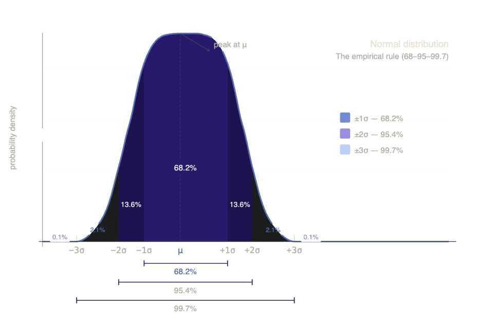
Standard Deviation — Measuring Consistency

Before we get to Mode, let us talk about standard deviation, because it connects beautifully to everything we have just discussed.

Standard deviation measures how spread out your numbers are from the mean. In simple terms, it tells you whether your values tend to stay close to the average or swing wildly away from it.

Using our bottle sales data again; 7, 10, 11, 12, 100, with a mean of 28, here is how far each value sits from that average:

Value Distance from Mean (28)

7 21 away

10 18 away

11 17 away

12 16 away

100 72 away — extreme outlier

Notice how most of the numbers are already somewhat far from the mean; but 100 is extraordinarily far. That one outlier drives the standard deviation up considerably.

What a High or Low Standard Deviation Means

Here is a simple comparison between two datasets that have the same mean but very different levels of consistency:

levels of consistency:

Dataset A is stable and predictable. Dataset B has the same average but wild swings; one exceptional day masks the reality of consistently low sales on all other days.

Why Companies Care About Standard Deviation

Standard deviation is so central to business improvement that it became the foundation of an entire management philosophy. In 1986, an engineer named Bill Smith at Motorola developed a concept called Six Sigma; built entirely around reducing variability in business processes. The idea: the less your processes deviate from the standard, the fewer errors, the lower the cost, and the better the customer experience.

Six Sigma is still widely used today, and Six Sigma-certified professionals are among the most sought after in large organisations globally. All of that, rooted in standard deviation.

One final note on a related term:

Variance is simply the square of the standard deviation. It is another way to express spread, and you will often see it mentioned alongside standard deviation in financial and statistical reports.

Mode — What Happens Most Often

Last but not least is the mode; and it is the simplest of the three measures. The mode is simply the value that appears most frequently in your dataset.

For example, if you look at your M-Pesa transaction history and you find that Ksh 100 appears more often than any other amount, then Ksh 100 is your modal spend. It is the amount you spend most often.

This can be an eye-opening measure. Perhaps that Ksh 100 is the cost of airtime you buy regularly, or a specific item you purchase out of habit. The mode puts a spotlight on your most repeated financial behaviour.

That said, the mode has its limitations. If your spending is highly varied and no single amount repeats significantly more than others, the mode may not tell you much. But in situations where clear patterns do exist, it becomes a very useful lens.

Bringing It All Together

Now you can see why these measures are not just academic concepts; they are practical tools for understanding your financial life.

When you know your mean daily spend, your median daily spend, and your standard deviation, you gain a layered picture of your financial behaviour. Are you consistent or erratic? Are a few big spending days distorting your average? What amount do you find yourself spending most often?

With that knowledge, you can take deliberate action. You might choose to budget using your mean as a target, or use your median as a more realistic benchmark. You can set a daily, weekly, or monthly spending limit directly at mpecunia/settings, and you will get a notification whenever you are approaching or have exceeded that limit.

Data-driven financial habits are not just for big corporations. They are for you too; and MPecunia is here to make that as simple as possible.

We hope this has been a worthwhile read. If you found it helpful, please leave a like and a comment, and let us know: what would you like to learn about next?